E102 - Hypothesis Testing
You are encouraged to familiarise yourself with a few topics prior to the exercise. The background section will provide you with some basic information and pointers. The exercise itself is designed to give you some practice in working with these concepts to give you a more intuitive grasp of them. The teacher will be able to supervise your during the exercise and explain the underlying theory if uncertainties remained during your preparation for the exercise.
Background
The following are topics you should try to familiarise yourself with prior to the exercise. Note that the serve as pointers and checks for your studies rather than as full instructional materials. It is expected that you internalised the theory of previous exercises.
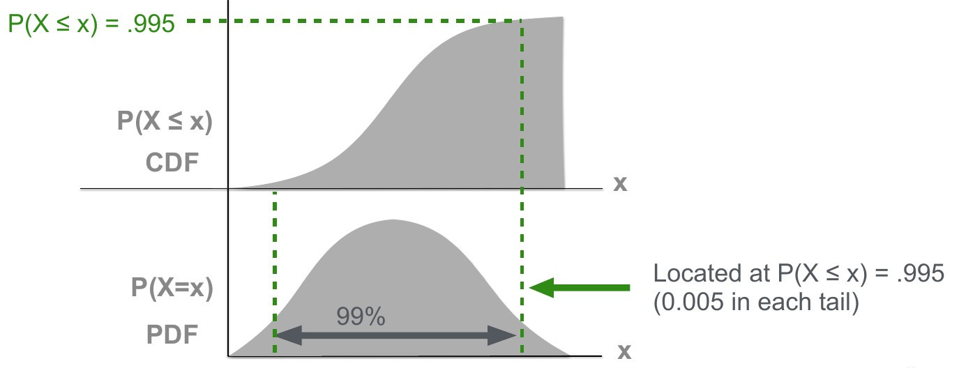
Topic 1: Familiarise yourself with probability density functions (PDFs), cumulatve distribution functions (CDFs) and the quantile (or percent point function). The figure shows the same data displayed as a PDF (\(P (X=x)\) ) and CDF (\(P (X=\bar{x})\) ). After your studies of the topics, you should understand what is displayed and labelled here.
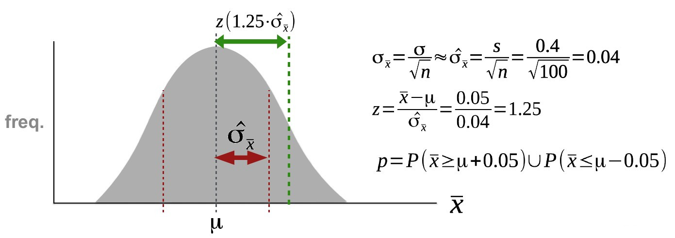
Topic 2: The next topics you should tacke are basic set notation, classic statistical hypothesis testing and one and two tailed testing. See if you can understand the following example after your studies:
“The DLR is investigating differences in albedo as clouds gain in thickness. Stratus clouds have an albedo of ca. 0.5, the observed albedo increase as they thicken up is 0.05, as picked up by 100 measurements. The sample standard deviation (s) is 0.4. Does thickness truly affect albedo?”
This scenario gives us:
Null hypothesis: Thickness has no effect; the mean is still 0.5 even after thickness increase. (\(H_0: \mu=0.5\) )
Alternative hypothesis: Thickness has an effect; the mean is no longer 0.5 after thickness increase. (\(H_A: \mu \ne 0.5\) )
If \(H_0: \mu=0.5\) is true, we can calculate the probability of getting a signal as extreme or even more extreme than the observed (0.05).
Finally:
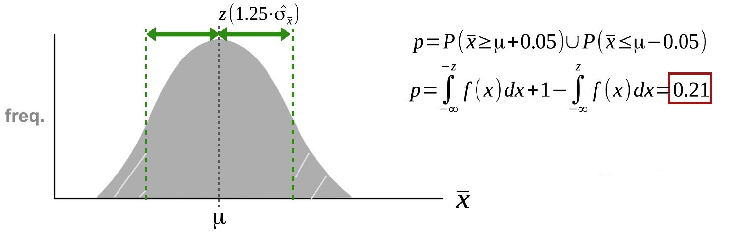
The probability (p) is too high for us to reject the null hypothesis \(H_0: \mu=0.5\) . With those specific sets of measurements and knowledge, we therefore cannot confidently say that thickness has an effect on albedo.
Exercise
Information
Topic |
|
|---|---|
Skills |
|
Hypothesis Testing: Temperatures near Antofagasta
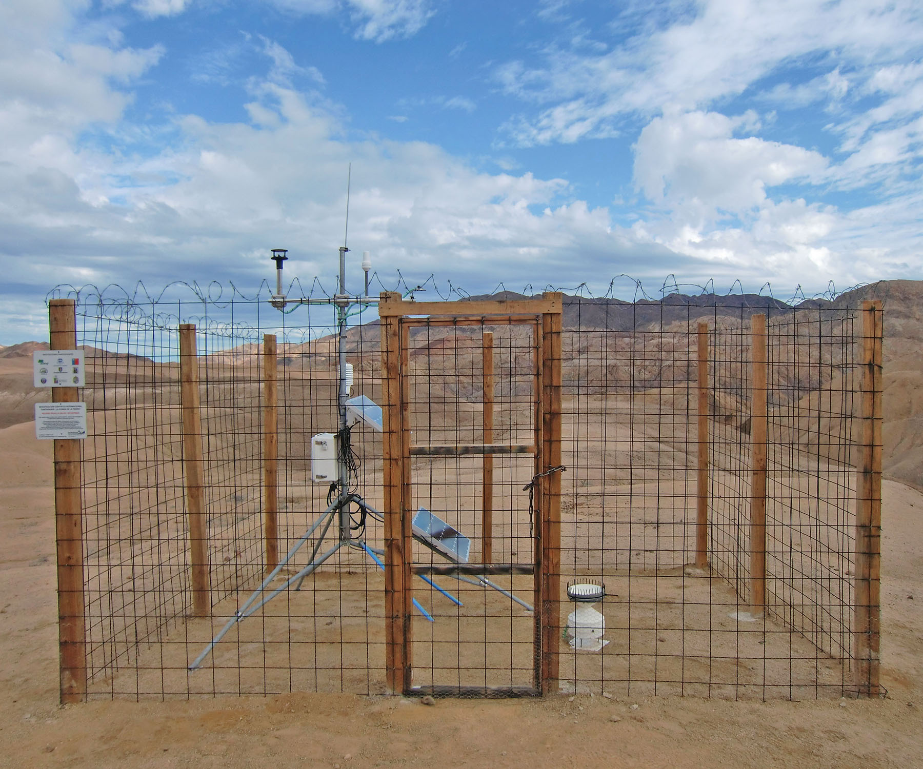
Weather station in Pan de Azucar National Park, ca. 200km south of Antofagasta. Records from different measurement systems flow into the interpolated observation-based datasets of re-analysis products. [photo: cc-by Kirstin Übernickel]
You are provided with an ERA-Interim re-analysis time series extracted for Antofagasta (Chile):
Regional climate models were forced with boundary conditions reflecting a low-emission-scenario state of technological and demographic developments. They simulated a climate for the 2070-2100. The model produced local January temperatures that have a mean of 23.6°C, and June temperatures with a mean of 17.2°C. You want to know if we see an increase in January and June temperatures near Antofagasta under the low-emission scenario. Using the dataset you are provided with, calculate the predicted temperature changes and determine if the signals are real or still within reasonable range of the observed temperature variability. Formulate testable hypothesess and apply your knowledge of statistical hypothesis testing, “p-values” and significance levels to answer this question.
HINT
You need models (PDF) to describe your null hypotheses. Think about how you would construct such a model for the problem you want to solve.
Warning
Late submissions won’t be accepted!