Building a Climate V

Coriolis Force

This lecture introduces the Coriolis force, the geostrophic balance and their implications for climate.

Information

Topics
Understand the Coriolis force and how to calculate it Understand the geostrophic balance and how it relates to wind speeds

Coriolis Force

The Coriolis force is an inertial force acting in a rotating frame of reference. It manifests itself when a body moves in a rotating reference frame and the body’s movement is not parallel to the angular velocity vector. The force acts on bodies that are already in motion. Therefore, it does not cause any winds, but does deflect winds. It acts perpendicular to the direction of motion (90° to the right in the northern hemisphere and 90° to the left in the southern hemisphere). Note that the Coriolis force also acts on objects not related to the atmosphere, so if you had a train travelling across latitudes in the northern hemisphere, you would theoretically expect to see greater wear on on side of the tracks, since the Coriolis force would act on the moving train to deflect it to the right. However, for Earth’s climate, those moving bodies are winds that get deflected. This deflection is sometimes referred to as the Coriolis effect. The Coriolis force can be calculated as follows:

\[\begin{equation} F_c = 2 · m · u · \Omega · sin(\phi) \end{equation}\]

where:

• \(F_c\) - coriolis force

• \(m\) - mass of the moving object

• \(u\) - velocity of the moving object

• \(\Omega\) - rotational rate

• \(\Phi\) - latitude

The rotational rate is planet-specific. Earth completes 1 rotation around its axis in a day. In other words, it travels its full circumference per day. If we convert days into seconds (1 d = 24 · 60 · 60 s), we can calculate Earth’s rotational rate in SI units:

\[\begin{equation} \Omega = \frac {2 · \pi (rad)} {60 · 60 · 24 (s)} = 2.27 · 10^{-5}s^{-1} \end{equation}\]

Note

A train with a mass of 10000 ton travels S-N at a speed of 120km/h. It is currently at 56.2°N. What is the Coriolis force acting on it? What would the Coriolis force be for the same train travelling on Mars?

Geostrophic Balance and Wind Speeds

The geostrophic balance (also known as geostrophic equilibrium) is a vector balance between the pressure gradient force and the Coriolis force. It is an important concept in atmospheric and oceanic sciences and helps us compute the speed of geostrophic currents. Geotrophic winds are theoretical wind currents that result from this balance.

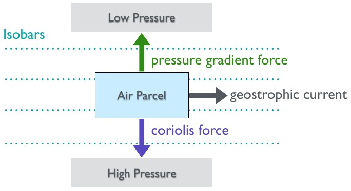
Geostrophic currents result from the geostrophic balance between the pressure gradient force an the Coriolis force.

For an air parcel moving across isobars, the pressure gradient force can be computed as:

\[\begin{equation} F_p = \frac {\Delta P}{\Delta D} · V = \nabla P · V \end{equation}\]

where:

• \(F_p\) - pressure gradient force

• \(\Delta_P\) - change in pressure

• \(\Delta_D\) - distance covered

• \(V\) - volume

Recall the equation for the Coriolis force:

\[\begin{equation} F_c = 2 · m · u · \Omega · sin(\phi) \end{equation}\]

We can write the m term (mass) as density times volume:

\[m = \rho · V\]

We can expand the geostrophic vector balance (\(F_p = F_c\) ) as:

\[\begin{equation} \nabla P · V = 2 · \rho · V · u · \Omega · sin(\phi) \end{equation}\]

Finally, we can rearrange the above to solve for velocity (\(u_g\) ), i.e. geostrophic current/wind speeds:

\[\begin{equation} u_g = \frac {\nabla P} {2 · \rho · \Omega · sin(\phi) } \end{equation}\]

In reality, ideal geostrophic winds are rare, since they are modified further by frictional forces (esp. where winds move close to the ground). However, they are good first approximations for extratropical regions.

Geostrophic Balance: Example Problem

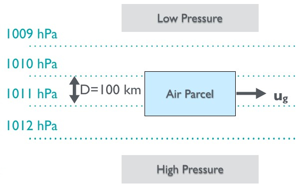
Geostrophic currents result from the geostrophic balance between the pressure gradient force an the Coriolis force.

Consider an air parcel in atmospheric pressure conditions that change by 1 hPa per 100km at 28°N. We can calculate the rate of change in pressure:

\[\begin{equation} \nabla P = \frac {1 · 10^2 Pa}{1 · 10^5m} = 1 · 10^{-3} Pa m^{-1} \end{equation}\]

We have already established the rotational rate and density of air (in a previous lecture). Using those values, we can calculate geostrophic wind speeds for our example:

\[\begin{equation} u_g = \frac {1 · 10^{-3} Pa m^{-1}} {2 · 1.2 kgm^{-3} · 2.27 · 10^{-5}s{-1} · sin(28.5) } \approx 18.7 ms^{-1} \end{equation}\]

Rossby Waves

Rossby waves, also known as planetary waves, are synoptic-scale atmospheric waves associated with the polar front and polar jet stream that separates cold polar air from warmer mid-latitude air [see “Building a climate VI”]. They result from the rotation of the planet, create fairly stable large-scale weather conditions in mid-high latitudes, and help transport heat from the tropics to the poles to solve the energy imbalance [see “Building a climate VI”].

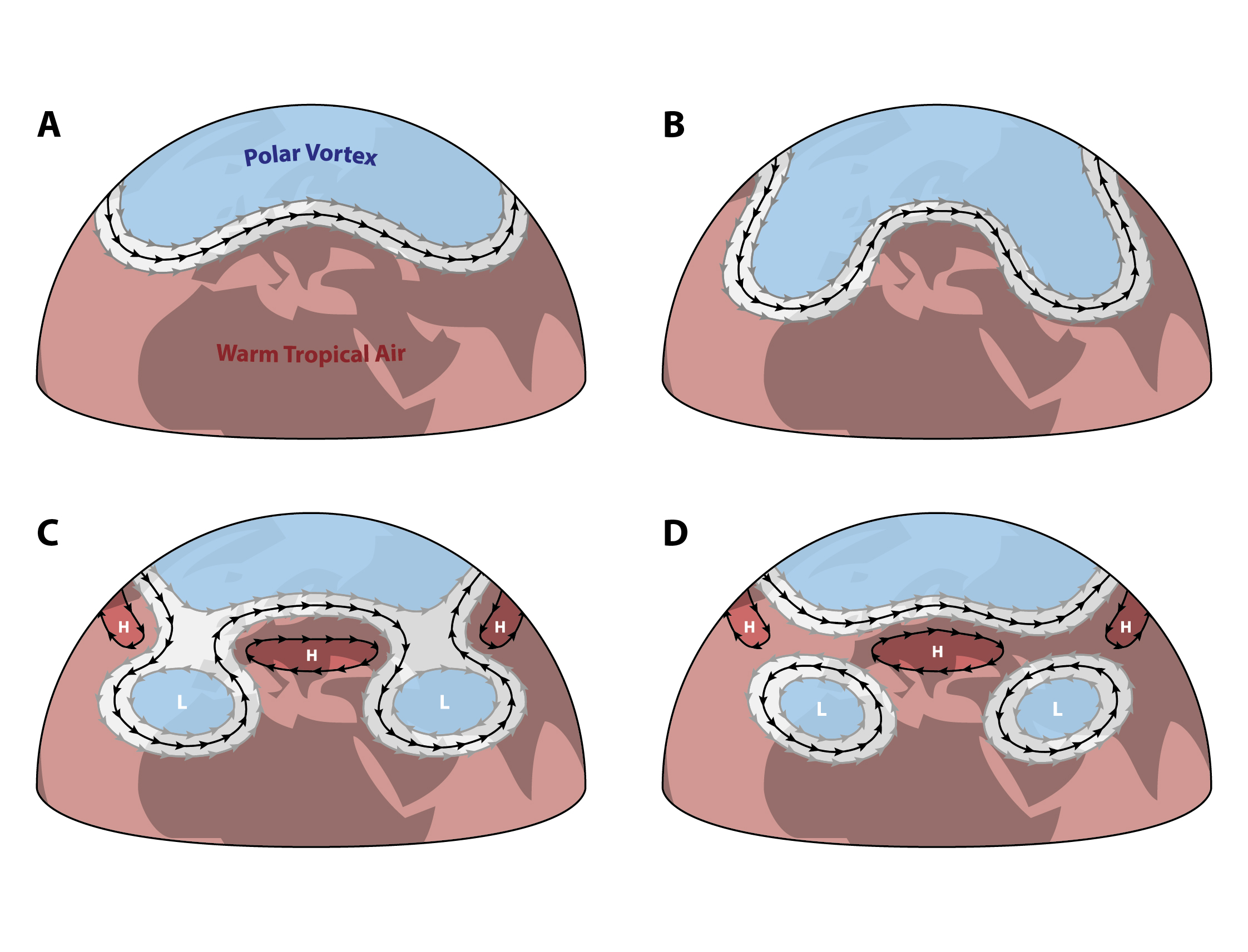
The evolution of Rossby waves, characterised by wave-like motions of the jet stream, and creation of high pressure cells (anti-cyclones) and low pressure cells (cyclones). [image: cc-by Lisa Rauschenbach]

This heat transport is enhanced when the amplitude increases and reduced when the amplitude is dampened. The wave amplitude can significantly vary, resulting in cold polar air penetrating far into the mid latitudes and creating anomalously cold weather. The protrusions created by increases in amplitude are “pinched off” to form high pressure cells (anti-cyclones) and low pressure cells (cyclones).

Cyclones, Anti-Cyclones and Geostrophic Winds

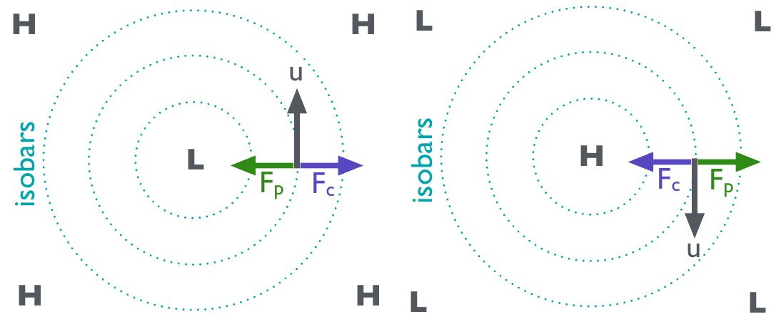
Left: Geostrophic winds follow a counterclockwise path in the Northern Hemisphere (and a clockwise path in the Southern Hemisphere) along the isobars of low pressure cells (cyclones).

Right: Geostrophic winds follow a a clockwise path in the Northern Hemisphere (and a counterclockwise path in the Southern Hemisphere) along the isobars of high pressure cells (anti-cyclones).

Cyclones are low pressure cells (usually denoted with an “L”) with high pressure around them.

Anti-Cyclones are high pressure cells (usually denoted with an “H”) with low pressure around them.

Recall our previous examples of an air parcel in atmospheric conditions with parallel isobars. In case of pressure cells, isobars are circular. This means that the pressure gradient force always acts towards the centre in case of a low pressure cell (cyclone) and away from the centre in case of a high pressure cell (anti-cyclone). We previously established that the Coriolis force acts in the opposite direction and the geostrophic wind vector is perpendicular to it. This remains the case with pressure cells. However, the direction of the pressure force, Coriolis force and wind vector changes as the air parcel’s position on the circular isobars changes, resulting in a circular motion of winds along the circular isobars.

Note

Place an air parcel onto different positions along one of the circular isobars and check this statement.

Small Excursion: Example Advection Schemes

So far, we have not written much of what we learned in differential form. Why? Because it is easier to understand this way. However, for most modelling applications, we cannot get around differential equations. This is a good time to introduce them.

Weather and climate models use Euler equations, the inviscid counterparts of Navier-Stokes equations, because frictional forces do not matter much for atmospheric flow.

These include an advection term to track the concentration of specific constituents of the atmosphere, such as water vapour or pollutants of concentration \(\Phi\) in a wind field \(u\) .

\[\begin{equation} \frac {\delta \Phi} {\delta t} + u · \nabla \Phi = source - sink \end{equation}\]

where t is time. Assuming that source = sink, we can write:

\[\begin{equation} \frac {\delta \Phi} {\delta t} + u · \frac {\delta \Phi} {\delta x} = 0 \end{equation}\]

where x is distance. Using a simple linear finite difference scheme (forward in time, backwards in space), we can write:

\[\begin{equation} \frac {\Phi_j^{n+1} - \Phi_j^{n}} {\Delta t} + u · \frac {\Phi_j^{n} - \Phi_{j-1}^{n}} {\Delta x} = 0 \end{equation}\]

Solving for concentration at the next time step and substituting the Courant number \(c = \frac {\Delta t}{\Delta x}\) :

\[\begin{equation} \Phi_j^{n+1} = \Phi_j^{n} - c · (\Phi_j^{n} - \Phi_{j-1}^{n}) \end{equation}\]

This allows us to compute concentration of the next time step in a FTBS (Forward Time Backward Space) advection scheme. We can also use an FTFS scheme:

\[\begin{equation} \Phi_j^{n+1} = \Phi_j^{n} - c · (\Phi_{j+1}^{n} - \Phi_{j}^{n}) \end{equation}\]

or an FTCS (Forward Time Centred Space) scheme:

\[\begin{equation} \Phi_j^{n+1} = \Phi_j^{n} - \frac {c}{2} · (\Phi_{j+1}^{n} - \Phi_{j-1}^{n}) \end{equation}\]

Note

While a real introduction to numerical modelling, differential equations and phase space is beyond the scope of this course, you should be aware that these topics are important for modelling atmospheric processes.